How to Set Up Your Market Buffer in Praxion

Case study: retiring at 62, Social Security at 67

A common pattern: you retire at 62 with about $1M in a 401(k), spend $5,000/month, and wait until 67 to claim Social Security. Monte Carlo may show 90%+ success — but the first five years can still run a 6%+ portfolio distribution rate because the plan must pull from the portfolio for living expenses and taxes on tax-deferred withdrawals.

A practical bridge: hold two years of portfolio pulls in cash (~$120k) plus three years of gap spending in short-term bonds (~$180k). That 30% defensive sleeve ($300k on $1M) is sized from spending, not age alone. Once Social Security starts, portfolio pulls often drop toward ~2.5% — and you can usually trim the defensive buckets and revisit equity.

In Praxion, the Income Planner buckets tab sizes this bridge automatically when your claim age is later than retirement. The Allocation Analyzer shows the implied defensive mix. Build the bridge 1–2 years before retirement when possible — sequence risk can start while you are still working if markets drop near your planned date.

Before you start

The buffer is most useful when:

• You are within 5–7 years of retirement (or already retired). Protection matters most around the transition.
• You have a meaningful brokerage balance to carve from. The buffer lives inside brokerage; it does not require a new account.
• Your monthly expenses are reasonably current — the buffer dollar amount is computed as months × monthly expenses.

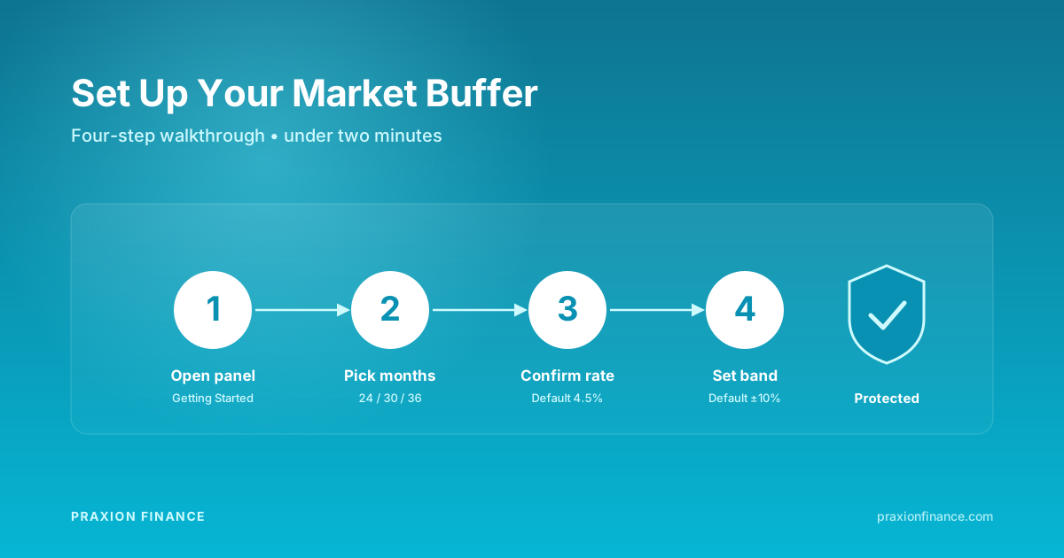
Step 1 — Open the cash reserve panel

Go to Getting Started → Investment Preferences (or jump directly to the profile editor and find the cash reserves section). Below the working-years and retirement-years cash reserve fields you'll find a teal panel titled 🛡️ Market buffer (optional).

Step 2 — Pick the number of months

The default is 0 (disabled). To enable, enter a positive number of months:

• 24 months — the most common setting. Suitable for moderate-risk-tolerance retirees.
• 30–36 months — more conservative. Preferred if you place a high value on stability or have inflexible spending needs.
• 12 months — light protection. Better than nothing if you have other defensive holdings outside brokerage.

As soon as you enter a positive number, the panel computes the dollar amount in real time: months × your monthly expenses. For someone spending $10,000 a month, a 24-month setting is a $240,000 buffer.

Step 3 — Confirm or adjust the return rate

The buffer return rate defaults to 4.5% — a realistic figure for T-bills, money-market funds, or ultra-short bond funds in a typical interest-rate environment. Adjust based on what you actually plan to hold:

• 3–4% — money-market funds, T-bills in a low-rate environment.
• 4.5–5.5% — ultra-short Treasury bond ETFs (SHV, BIL) in a normal-rate environment.
• 5.5–6.5% — short-duration corporate or muni bond funds. Slightly more volatility, slightly higher yield.

Step 4 — Leave the maintenance band at default (or tighten it)

The maintenance band defaults to ±10%. The engine only rebalances when the buffer drifts more than 10% above or below its target. Tighter bands (±5%) mean more frequent rebalancing; looser bands (±15%) let the buffer ride longer.

For most users the 10% default is fine. If you want a smoother buffer trajectory, set it to 5%. There is no rebalancing tax cost — all transfers are internal accounting within one brokerage account.

Save and verify

Save your profile. The engine starts using the new settings on your next projection refresh. Two ways to confirm it's working:

• Year-by-year table at Projection Details. Look for the bufferBalance column. Starting at your first retirement year, you should see a non-zero value that grows at roughly your configured buffer rate.
• Dashboard cash card at Dashboard. The card now displays a 🛡️ note: “Plan includes a ~$Y market buffer (Z months) carved from brokerage at retirement.”

What to expect in the numbers

In a deterministic projection (no crashes), the buffer typically reduces your final-balance estimate by a few percentage points. That's the cost of insurance — the buffer earns less than equities. You're looking at the “everything goes right” case where the protection wasn't needed.

Where the buffer shines is the Monte Carlo / stress-test view. With buffer enabled, plan success rate under random scenarios increases — typically 5–15 percentage points for a 24-month buffer, more for 30–36 months. That delta is the insurance premium delivering its protection.

If you change your mind

Setting buffer months back to 0 disables the feature entirely. The engine reverts to treating brokerage as a single equity sleeve. There is no migration step or data loss — the buffer is a model toggle, not a real-world account.

In real life, of course, if you actually moved money into short-duration bonds for the buffer, you'll need to move it back out if you decide to disable. The model and the real-world implementation are separate decisions.